2 Chapter 9: Factor Analysis

2.1 Overview of FA

The essential purpose of FA: to describe the covariance relationships among many variables in terms of a few understanding, but unobservable, random quantities called factors.
Basic objective 1: to determine whether the \(p\) variables exhibit patterns of relationship with each other such that
- the variables can be partitioned into, say, \(m\) subsets (\(m<p\)),
- each subset consists of a group of variables tending to be more highly related to others within the subset than to those in other subsets.
Example:
- Correlations from the group of test scores in classics, French, English, mathematics, and music collected by Spearman suggested an underlying “intelligence” factor.
- A second group of variables: physical-fitness scores, if available, might correspond to another factor.
- FA seeks to confirm such type of structure.
Basic objective 2: to derive, create, or develop a new set of uncorrelated variables
- the new variables are called underlying factors or underlying characteristics
- we hope the new variables give a better understanding of the data being analyzed
- the new variables can then be used in future analyses of the data
The factor analysis model assumes there is a smaller set of uncorrelated variables that, in some sense, drives or controls the values of the variables that are actually being measured.
The difference between PCA and FA: PCA is a linear combination of variables; Factor Analysis is a measurement model of a latent variable.

2.2 Warnings

If the original variables are already uncorrelated, then there is little reason to consider performing a FA.
Criticism on FA:
- There is no unique solution to FA.
- Subjective decisions are made for determining
  - the number of underlying factors
  - how they are created
  - how they should be interpreted
  - how individuals in the sample should be evaluated on the
  - new variables

2.3 The Orthogonal Factor Model

\(\vec X\) is a \(p\)-dimensional random vector \(\sim (\vec \mu, \mathbf{\Sigma})\).

The factor analysis model is \[X_i - \mu_i=l_{i1}F_1+l_{i2}F_2+\dots+l_{im}F_m+\epsilon_i,\]

\(X_i\) is the \(i\)-th component of \(\vec X\).
\(F_1, F_2, \dots, F_m\) are called common factors
\(\epsilon_1, \epsilon_2, \dots, \epsilon_p\) are called errors or specific factors
\(l_{ij}\) is called the loading of the \(i\)th variable on the \(j\)th factor

or in matrix notation:

\[\underset{(p\times 1)}{\vec X - \vec \mu}=\underset{(p\times m)}{\mathbf{L}}\underset{(m\times 1)}{\vec F}+\underset{(p\times 1)}{\vec \epsilon}\]

\(\mathbf{L}\): matrix of factor loadings

2.3.1 Orthogonal Factor Model with \(m\) Common Factors

\[\underset{(p\times 1)}{\vec X}=\underset{(p\times 1)}{\vec \mu}+\underset{(p\times m)}{\mathbf{L}}\underset{(m\times 1)}{\vec F}+\underset{(p\times 1)}{\vec \epsilon}\]

\(\mu_i\): mean of variable \(i\)

\(\epsilon_i\): \(i\)th specific factor

\(F_j\): \(j\)th common factor

\(l_{ij}\): loading of the \(i\)th variable on the \(j\)th factor

Assumptions:

\(\vec F\) and \(\vec \epsilon\) are independent

\(E(\vec F)=\vec 0, Cov(\vec F)=\mathbf{I}\)

\(E(\vec \epsilon)=\vec 0, Cov(\vec \epsilon)=\mathbf{\Psi}\), where \(\mathbf{\Psi}\) is a diagonal matrix

2.3.2 Covariance Structure of \(\vec X\) under the Orthogonal Factor Model

\(\mathbf{\Sigma}=Cov(\vec X) = \mathbf{L}\mathbf{L}'+\mathbf{\Psi}\) (factor analysis equation)
\(Cov(\vec X, \vec F) = \mathbf{L}\)

Then, we can decompose the variance of the \(i\)th variable into two parts:

\(i\)th communality: \(h_i^2=l_{i1}^2+l_{i2}^2+\dots+l_{im}^2\)
\(i\)th uniqueness or specific variance: \(\psi_i\)

\[Var(X_i)=\sigma_{ii}=h_i^2+\psi_i, i=1,2,\dots,p\]

To determine if \(\vec F, \mathbf{L}\) and \(\vec \epsilon\) exist such that \(\vec X- \vec \mu= \mathbf{L}\vec F+\vec \epsilon\), we try to find \(\mathbf{L}\) and \(\mathbf{\Psi}\) so that the factor analysis equation holds: \(\mathbf{\Sigma}=\mathbf{L}\mathbf{L}'+\mathbf{\Psi}\).
Remark: In practice, FA procedures are almost always applied to \(Z\) scores and to the correlation matrix \(\mathbf{\rho}\).
Example 9.1: p. 484. Verifying \(\mathbf{\Sigma}=\mathbf{L}\mathbf{L}'+\mathbf{\Psi}\) for two factors
Example 9.2: p. 486. Nonexistence of a proper solution to the FA equation

2.3.3 Nonuniqueness of the Factors

For any \(m \times m\) orthogonal matrix \(\mathbf{T}\), we have

\[\mathbf{\Sigma}=\mathbf{L}\mathbf{L}'+\mathbf{\Psi}=\mathbf{LTT'L'}+\mathbf{\Psi}=\mathbf{(LT)}\mathbf{(LT)}'+\mathbf{\Psi}\] and \[Cov(\mathbf{T}'\vec F)=\mathbf{T}'\mathbf{T}=\mathbf{I}.\]

That is, if \(\mathbf{L}\) is a loading matrix, then \(\mathbf{L}^*=\mathbf{LT}\) is also a loading matrix for factors \(\vec F^*=\mathbf{T}'\vec F\), which satisfies

\[\mathbf{L}^*\vec F^*=\mathbf{L}\vec F.\]

Hence, the factor loading matrix \(\mathbf{L}\) is not unique.

2.4 9.3 Methods of Estimation

Question: Does the FA model with a small number of factors, adequately represent the data?

Solution: verify the covariance relationship:

\(\mathbf{\Sigma}=Cov(\vec X) = \mathbf{L}\mathbf{L}'+\mathbf{\Psi}\)
\(Cov(\vec X, \vec F) = \mathbf{L}\)

Parameters in the FA model: the factor loadings \(l_{ij}\) and specific variances \(\psi_{i}\).
Two of the most popular methods of parameter estimation
- the principal component (and the related principal factor) method
- the maximum likelihood method.

2.4.1 The Principal Component (and Principal Factor) Method

The spectral decomposition:

\[ \begin{aligned} \mathbf{\Sigma} & = \lambda_1\vec e_1\vec e_1'+\dots+\lambda_p\vec e_p\vec e_p'\\ &=\begin{bmatrix} \sqrt{\lambda_1}\vec e_1& \dots& \sqrt{\lambda_p}\vec e_p \end{bmatrix} \begin{bmatrix} \sqrt{\lambda_1}\vec e_1\\ \dots\\ \sqrt{\lambda_p}\vec e_p \end{bmatrix} \end{aligned} \]

where \(\lambda_1\ge \lambda_2\ge\dots\lambda_p\ge0\).

Neglecting the last \(p-m\) small eigenvalues and allowing for specific factors, we have the following approximation:

\[ \begin{aligned} \mathbf{\Sigma} & \approx \mathbf{L}\mathbf{L}'+\mathbf{\Psi}\\ &=\begin{bmatrix} \sqrt{\lambda_1}\vec e_1& \dots& \sqrt{\lambda_m}\vec e_m \end{bmatrix} \begin{bmatrix} \sqrt{\lambda_1}\vec e_1\\ \dots\\ \sqrt{\lambda_m}\vec e_m \end{bmatrix} + \begin{bmatrix} \psi_{1} & 0 & \dots & 0 \\ 0 & \psi_{2} & \dots & 0 \\ \vdots & \vdots & \ddots& \vdots \\ 0 & 0 & \dots & \psi_{p} \end{bmatrix} \end{aligned} \]

2.4.1.1 Principle Component Solution of the Factor Model

The matrix of estimated factor loadings \(\{\tilde{l}_{ij}\}\):

\[\widetilde{\mathbf{L}}=\begin{bmatrix} \sqrt{\hat\lambda_1}\hat{\vec e_1}& \dots& \sqrt{\hat\lambda_m}\hat{\vec e_m} \end{bmatrix},\]

where \(({\hat\lambda_i}\hat{\vec e_i})\) are eigenvalue-eigenvector pairs of the sample covariance matrix \(\mathbf{S}\), and \(\hat\lambda_1\ge \hat\lambda_2\ge\dots\hat\lambda_p\ge0\).

The estimated specific variances are provided by the diagonal elements of \(\mathbf{S} - \widetilde{\mathbf{L}}\widetilde{\mathbf{L}}'\):

\[\widetilde{\mathbf{\Psi}}=\begin{bmatrix} \widetilde\psi_{1} & 0 & \dots & 0 \\ 0 & \widetilde\psi_{2} & \dots & 0 \\ \vdots & \vdots & \ddots& \vdots \\ 0 & 0 & \dots & \widetilde\psi_{p} \end{bmatrix} \text{ with } \widetilde\psi_{i}=s_{ii} - \sum_{j=1}^m\tilde{l}_{ij}^2,\]

Communalities are estimated as \(\tilde{h}_{i}^2=\sum_{j=1}^m\tilde{l}_{ij}^2\)
The residual matrix: \(\mathbf{S} - (\widetilde{\mathbf{L}}\widetilde{\mathbf{L}}' + \widetilde{\mathbf{\Psi}})\).
The contribution to the total sample variance from the \(j\)th factor: \(\sum_{i=1}^p\tilde{l}_{ij}^2=\hat\lambda_i\)

2.4.1.2 Example 9.3 (p. 491)

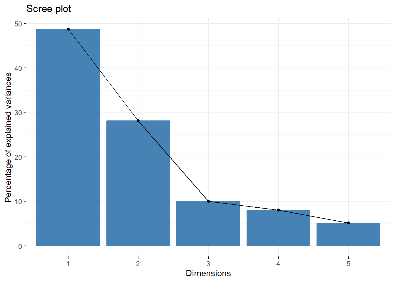
2.4.1.3 Example 9.4 (p. 493, FA of stock-price data)

X <- as.matrix(read.table("dataset/T8-4.DAT"))
colnames(X) <- c("JPM", "Citi", "WellsF", "Shell", "Exxon")
head(X)
#>             JPM       Citi     WellsF      Shell      Exxon
#> [1,]  0.0130338 -0.0078431 -0.0031889 -0.0447693  0.0052151
#> [2,]  0.0084862  0.0166886 -0.0062100  0.0119560  0.0134890
#> [3,] -0.0179153 -0.0086393  0.0100360  0.0000000 -0.0061428
#> [4,]  0.0215589 -0.0034858  0.0174353 -0.0285917 -0.0069534
#> [5,]  0.0108225  0.0037167 -0.0101345  0.0291900  0.0409751
#> [6,]  0.0101713 -0.0121978 -0.0083768  0.0137083  0.0029895

# PCA based on the spectral decomposition
# cor=T: standardized variables/correlation matrix
X.pc <- princomp(X, cor=T)
library(factoextra)
#> Loading required package: ggplot2
#> Welcome! Want to learn more? See two factoextra-related books at https://goo.gl/ve3WBa
fviz_eig(X.pc)


R <- cor(X)
ed <- eigen(R)
lambda <- ed$values
lambda
#> [1] 2.4372731 1.4070127 0.5005127 0.4000316 0.2551699
ei <- ed$vectors

L.all <- ei %*% diag(sqrt(lambda)) 

# m = 2
m <- 2
L <- L.all[, 1:m] # estimated factor loadings
h2 <- rowSums(L^2) # communalities
psi <- 1 - h2 # estimated specific variances

df <- data.frame(variable=c(colnames(X)),
                 F1=L[, 1],
                 F2=L[, 2],
                 h2=h2,
                 psi=psi)
df[sapply(df, is.numeric)] <- round(df[sapply(df, is.numeric)], 3)
df
#>   variable     F1     F2    h2   psi
#> 1      JPM -0.732  0.437 0.727 0.273
#> 2     Citi -0.831  0.280 0.770 0.230
#> 3   WellsF -0.726  0.374 0.667 0.333
#> 4    Shell -0.605 -0.694 0.847 0.153
#> 5    Exxon -0.563 -0.719 0.834 0.166

Residual <- R - L %*% t(L) - diag(psi)
Residual
#>                JPM        Citi       WellsF        Shell
#> JPM     0.00000000 -0.09884073 -0.184513342 -0.025317756
#> Citi   -0.09884073  0.00000000 -0.134323655  0.014310342
#> WellsF -0.18451334 -0.13432365  0.000000000  0.002794963
#> Shell  -0.02531776  0.01431034  0.002794963  0.000000000
#> Exxon   0.05580220 -0.05378426  0.005960127 -0.155835955
#>               Exxon
#> JPM     0.055802201
#> Citi   -0.053784258
#> WellsF  0.005960127
#> Shell  -0.155835955
#> Exxon   0.000000000

In this example, the first factor might be called market factor, and the second factor might be called industry factor.

2.4.2 The Maximum likelihood Method

We assume normality, and maximize the likelihood over \(\vec \mu\) and \(\mathbf{\Sigma}\), subject to \(\mathbf{\Sigma}=\mathbf{L}\mathbf{L}'+\mathbf{\Psi}\).
It is desirable to make \(\mathbf{L}\) well defined by imposing the computationally convenient uniqueness condition:

\[\mathbf{L}'\mathbf{\Psi}^{-1}\mathbf{L}=\mathbf{\Delta}=diag\{\delta_1\ge\dots\ge\delta_m\}\]

We require that there are less parameters in the restricted FA model than in the unrestricted model.
- number of parameters in the restricted FA model (\(\mathbf{L}\mathbf{L}'+\mathbf{\Psi}\)): \(p+pm-(m-1)m/2\)
- number of parameters in the unrestricted model (\(\mathbf{\Sigma}\)): \(p(p+1)/2\)

2.4.2.1 Example 9.5 (Factor analysis of stock-price data using the maximum likelihood method)

X <- as.matrix(read.table("dataset/T8-4.DAT"))
colnames(X) <- c("JPM", "Citi", "WellsF", "Shell", "Exxon")
head(X)
#>             JPM       Citi     WellsF      Shell      Exxon
#> [1,]  0.0130338 -0.0078431 -0.0031889 -0.0447693  0.0052151
#> [2,]  0.0084862  0.0166886 -0.0062100  0.0119560  0.0134890
#> [3,] -0.0179153 -0.0086393  0.0100360  0.0000000 -0.0061428
#> [4,]  0.0215589 -0.0034858  0.0174353 -0.0285917 -0.0069534
#> [5,]  0.0108225  0.0037167 -0.0101345  0.0291900  0.0409751
#> [6,]  0.0101713 -0.0121978 -0.0083768  0.0137083  0.0029895

m <- 2
# Maximum likelihood solution
# The R function factanal() computes the mle on the basis of the sample correlation matrix R.
fit.mle <- factanal(X, m, rotation = "none") # agrees with textbook (almost); "varimax" is the default
fit.mle
#> 
#> Call:
#> factanal(x = X, factors = m, rotation = "none")
#> 
#> Uniquenesses:
#>    JPM   Citi WellsF  Shell  Exxon 
#>  0.417  0.275  0.542  0.005  0.530 
#> 
#> Loadings:
#>        Factor1 Factor2
#> JPM     0.121   0.754 
#> Citi    0.328   0.786 
#> WellsF  0.188   0.650 
#> Shell   0.997         
#> Exxon   0.685         
#> 
#>                Factor1 Factor2
#> SS loadings      1.622   1.610
#> Proportion Var   0.324   0.322
#> Cumulative Var   0.324   0.646
#> 
#> Test of the hypothesis that 2 factors are sufficient.
#> The chi square statistic is 1.97 on 1 degree of freedom.
#> The p-value is 0.16

# check: 
colSums(fit.mle$loadings^2)
#>  Factor1  Factor2 
#> 1.622061 1.609847

L <- fit.mle$loadings
L
#> 
#> Loadings:
#>        Factor1 Factor2
#> JPM     0.121   0.754 
#> Citi    0.328   0.786 
#> WellsF  0.188   0.650 
#> Shell   0.997         
#> Exxon   0.685         
#> 
#>                Factor1 Factor2
#> SS loadings      1.622   1.610
#> Proportion Var   0.324   0.322
#> Cumulative Var   0.324   0.646
Psi <- diag(fit.mle$uniquenesses)
round(t(L)%*%solve(Psi)%*%L,4) # diagonal
#>          Factor1 Factor2
#> Factor1 200.3689  0.0000
#> Factor2   0.0000  4.4049
resids.mle <- R - (L%*%t(L) + Psi) # much smaller than residsual from the PC solution
resids.mle
#>                  JPM          Citi        WellsF
#> JPM     1.055860e-07  7.496780e-06 -2.564223e-03
#> Citi    7.496780e-06  3.255672e-08  1.608871e-03
#> WellsF -2.564223e-03  1.608871e-03  5.157370e-08
#> Shell  -3.325561e-04  2.116218e-04 -9.518792e-06
#> Exxon   5.198222e-02 -3.307885e-02  5.547153e-04
#>                Shell         Exxon
#> JPM    -3.325561e-04  5.198222e-02
#> Citi    2.116218e-04 -3.307885e-02
#> WellsF -9.518792e-06  5.547153e-04
#> Shell  -1.559500e-06  1.218853e-04
#> Exxon   1.218853e-04  2.670491e-07
round(resids.mle, 4)
#>            JPM    Citi  WellsF  Shell   Exxon
#> JPM     0.0000  0.0000 -0.0026 -3e-04  0.0520
#> Citi    0.0000  0.0000  0.0016  2e-04 -0.0331
#> WellsF -0.0026  0.0016  0.0000  0e+00  0.0006
#> Shell  -0.0003  0.0002  0.0000  0e+00  0.0001
#> Exxon   0.0520 -0.0331  0.0006  1e-04  0.0000

The ML method suggests that the first factor might be called banking factor, and the second factor might be called oil industry factor.

2.4.3 A Large Sample Test for the Number of Common Factors

In the result of Example 9.5, there is a likelihood ratio test for \(m\):

“Test of the hypothesis that 2 factors are sufficient. The chi square statistic is 1.97 on 1 degree of freedom. The p-value is 0.16.”

2.4.3.1 likelihood ratio test for \(m\)

From Equation (4-18), Result 5.2, and Supplement 9A in the textbook, we have the likelihood ratio statistic for \(H_0: \mathbf{\Sigma}=\mathbf{L}\mathbf{L}'+\mathbf{\Psi}\):

\[-2\ln\Lambda = n\ln\bigg(\frac{|\hat{\mathbf{L}} \hat{\mathbf{L}}'+\hat{\mathbf{\Psi}}|}{|(n-1)/n\mathbf{S}|}\bigg).\]

The Bartlett’s correlation:

\[(n-1-(2p+4m+5)/6)\ln\bigg(\frac{|\hat{\mathbf{L}} \hat{\mathbf{L}}'+\hat{\mathbf{\Psi}}|}{|(n-1)/n\mathbf{S}|}\bigg)\sim \chi^2_{[(p-m)^2]-(p+m)]/2}\]

2.5 9.4 Factor Rotation \(\mathbf{L}^*=\mathbf{LT}\)

We have shown that the FA model is invariant under orthogonal transformation (the loadings solution is not unique.)
We attempt to choose a transformation to make the factors more interpreble. The loadings on each particular factor can be easily split into interpreble groups, which means for each \(j\), \(\hat{l}_{ij}\) should be highly varied.

2.5.1 varimax criterion

Define \(\tilde{l}_{ij}^*=\dfrac{\hat{l}_{ij}^*}{\hat h_i}\). Then, the varimax criterion selects the orthogonal transformation \(\mathbf{T}\) to maximize

\[V=\dfrac{1}{p}\sum_{j=1}^m\Big[\sum_{i=1}^p\tilde{l}_{ij}^{*4} -\dfrac{(\sum_{i=1}^p\tilde{l}_{ij}^{*2})^2}{p} \Big].\]

2.5.2 Example 9.9 (p. 508, self-study, SAS program)

factor 1: nutritional factor; factor 2: taste factor

2.5.3 Example 9.10 (Rotated loading for the stock-price data)

X <- as.matrix(read.table("dataset/T8-4.DAT"))
colnames(X) <- c("JPM", "Citi", "WellsF", "Shell", "Exxon")
head(X)
#>             JPM       Citi     WellsF      Shell      Exxon
#> [1,]  0.0130338 -0.0078431 -0.0031889 -0.0447693  0.0052151
#> [2,]  0.0084862  0.0166886 -0.0062100  0.0119560  0.0134890
#> [3,] -0.0179153 -0.0086393  0.0100360  0.0000000 -0.0061428
#> [4,]  0.0215589 -0.0034858  0.0174353 -0.0285917 -0.0069534
#> [5,]  0.0108225  0.0037167 -0.0101345  0.0291900  0.0409751
#> [6,]  0.0101713 -0.0121978 -0.0083768  0.0137083  0.0029895

R = cor(X)

m <- 2
# Maximum likelihood solution
# The R function factanal() computes the mle on the basis of the sample correlation matrix R.
fit.mle <- factanal(X, m, rotation = "none") # agrees with textbook (almost); "varimax" is the default

# Rotations 
fit.mle # mle; no rotation
#> 
#> Call:
#> factanal(x = X, factors = m, rotation = "none")
#> 
#> Uniquenesses:
#>    JPM   Citi WellsF  Shell  Exxon 
#>  0.417  0.275  0.542  0.005  0.530 
#> 
#> Loadings:
#>        Factor1 Factor2
#> JPM     0.121   0.754 
#> Citi    0.328   0.786 
#> WellsF  0.188   0.650 
#> Shell   0.997         
#> Exxon   0.685         
#> 
#>                Factor1 Factor2
#> SS loadings      1.622   1.610
#> Proportion Var   0.324   0.322
#> Cumulative Var   0.324   0.646
#> 
#> Test of the hypothesis that 2 factors are sufficient.
#> The chi square statistic is 1.97 on 1 degree of freedom.
#> The p-value is 0.16
fit.mle.r = factanal(X, m, rotation = "varimax")
fit.mle.r  
#> 
#> Call:
#> factanal(x = X, factors = m, rotation = "varimax")
#> 
#> Uniquenesses:
#>    JPM   Citi WellsF  Shell  Exxon 
#>  0.417  0.275  0.542  0.005  0.530 
#> 
#> Loadings:
#>        Factor1 Factor2
#> JPM    0.763          
#> Citi   0.819   0.232  
#> WellsF 0.668   0.108  
#> Shell  0.113   0.991  
#> Exxon  0.108   0.677  
#> 
#>                Factor1 Factor2
#> SS loadings      1.725   1.507
#> Proportion Var   0.345   0.301
#> Cumulative Var   0.345   0.646
#> 
#> Test of the hypothesis that 2 factors are sufficient.
#> The chi square statistic is 1.97 on 1 degree of freedom.
#> The p-value is 0.16
# Bank stocks (variables 1,2,3) load heavily on factor 1, much less so on factor 2;
# oil stocks load heavily on factor 2, much less so on factor 1.

# or you can use varimax() function to rotate the loadings
rotate = varimax(loadings(fit.mle))  # identical to fit.mle.r, but labeling of factors is reversed
rotate
#> $loadings
#> 
#> Loadings:
#>        Factor1 Factor2
#> JPM            0.763  
#> Citi   0.232   0.819  
#> WellsF 0.108   0.668  
#> Shell  0.991   0.113  
#> Exxon  0.677   0.108  
#> 
#>                Factor1 Factor2
#> SS loadings      1.507   1.725
#> Proportion Var   0.301   0.345
#> Cumulative Var   0.301   0.646
#> 
#> $rotmat
#>            [,1]      [,2]
#> [1,]  0.9927706 0.1200276
#> [2,] -0.1200276 0.9927706

2.6 9.5 Factor Scores (Estimation of the common factors \(\vec f\))

Factor scores are estimates of values of the unobserved random factor vectors \(\vec F\), not estimates of unknown parameters.

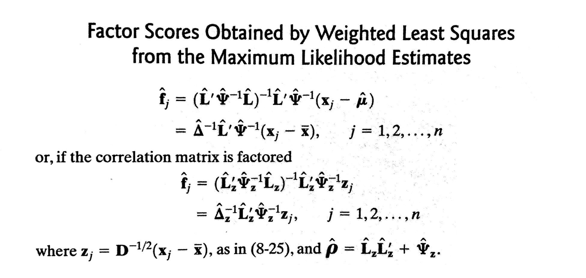
2.6.1 The Weighted Least Square Method (‘Bartlett’ scores in R when using factanal())

Bartlett proposed choosing the estimates \(\hat{\vec f}\) of \(\vec f\) to minimize the sum of the squares of the errors, which is weighted by the reciprocal of their variances:

\[\sum_{i=1}^p\dfrac{\epsilon_i^2}{\psi_i}=\vec \epsilon'\mathbf{\Psi}^{-1}\vec \epsilon=(\vec x - \vec \mu - \mathbf{L}\vec f)'\mathbf{\Psi}^{-1}(\vec x - \vec \mu - \mathbf{L}\vec f).\]

Comment: For the principle component solution, we generate factor scores using an unweighted (ordinary) least squares procedure (assume that the specific variances \(\psi_i\) are equal or nearly equal.)

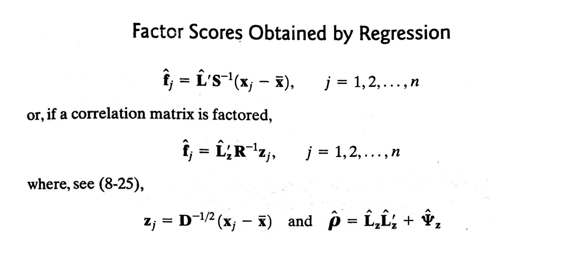
2.6.2 The Regression Method (‘regression’ scores in R when using factanal())

Regression formula: \(\vec F \sim \vec x\)
Under the normality assumption, \(\vec X - \vec \mu\) and \(\vec F\) are jointly normal:

\[ \begin{bmatrix} \vec X - \vec \mu \\ \vec F \end{bmatrix} = N_{p+m} \Bigg(\vec 0, \begin{bmatrix} \mathbf{\Sigma} = \mathbf{L}\mathbf{L}'+\mathbf{\Psi} & \mathbf{L} \\ \mathbf{L}' & \mathbf{I} \end{bmatrix}\Bigg) \]

By Result 4.6, the conditional distribution of \(\vec F|\vec x\) is multivariate normal with

\[E(\vec F|\vec x) = \mathbf{L}'\mathbf{\Sigma}^{-1}(\vec X - \vec \mu)=\mathbf{L}'(\mathbf{L}\mathbf{L}'+\mathbf{\Psi})^{-1}(\vec X - \vec \mu)\]

2.6.2.1 The stock-price data Example for factor scores

X <- as.matrix(read.table("dataset/T8-4.DAT"))
colnames(X) <- c("JPM", "Citi", "WellsF", "Shell", "Exxon")
head(X)
#>             JPM       Citi     WellsF      Shell      Exxon
#> [1,]  0.0130338 -0.0078431 -0.0031889 -0.0447693  0.0052151
#> [2,]  0.0084862  0.0166886 -0.0062100  0.0119560  0.0134890
#> [3,] -0.0179153 -0.0086393  0.0100360  0.0000000 -0.0061428
#> [4,]  0.0215589 -0.0034858  0.0174353 -0.0285917 -0.0069534
#> [5,]  0.0108225  0.0037167 -0.0101345  0.0291900  0.0409751
#> [6,]  0.0101713 -0.0121978 -0.0083768  0.0137083  0.0029895

m <- 2
# WLS scores 
fit.ml.WLS.r = factanal(X, m, rotation = "varimax", scores = "Bartlett") 

# Regression scores 
fit.ml.reg.r = factanal(X, m, rotation = "varimax", scores = "regression")
fit.ml.reg.r
#> 
#> Call:
#> factanal(x = X, factors = m, scores = "regression", rotation = "varimax")
#> 
#> Uniquenesses:
#>    JPM   Citi WellsF  Shell  Exxon 
#>  0.417  0.275  0.542  0.005  0.530 
#> 
#> Loadings:
#>        Factor1 Factor2
#> JPM    0.763          
#> Citi   0.819   0.232  
#> WellsF 0.668   0.108  
#> Shell  0.113   0.991  
#> Exxon  0.108   0.677  
#> 
#>                Factor1 Factor2
#> SS loadings      1.725   1.507
#> Proportion Var   0.345   0.301
#> Cumulative Var   0.345   0.646
#> 
#> Test of the hypothesis that 2 factors are sufficient.
#> The chi square statistic is 1.97 on 1 degree of freedom.
#> The p-value is 0.16

out = cbind(fit.ml.WLS.r$scores, fit.ml.reg.r$scores) # use varimax
colnames(out) = c("wls.r.F1", "wls.r.F2", "reg.r.F1", "reg.r.F2")
out[1:10,] # There are n = 103 rows
#>          wls.r.F1    wls.r.F2    reg.r.F1    reg.r.F2
#>  [1,]  0.25089936 -1.85367070  0.16535864 -1.83427398
#>  [2,]  0.44303382  0.24787783  0.36753184  0.25550919
#>  [3,] -0.48078772 -0.09835680 -0.39519052 -0.10792854
#>  [4,]  0.79921292 -1.31497895  0.62520403 -1.28789064
#>  [5,] -0.09859658  0.95881635 -0.06003873  0.94945235
#>  [6,] -0.47081640  0.41285165 -0.37607023  0.39962913
#>  [7,]  0.95854964  0.88173946  0.80260447  0.89563925
#>  [8,]  1.03632812 -0.03557662  0.84651321 -0.01307322
#>  [9,] -1.07061981 -1.14851602 -0.89995399 -1.16280345
#> [10,]  0.55016716 -0.97789250  0.42882250 -0.95869583

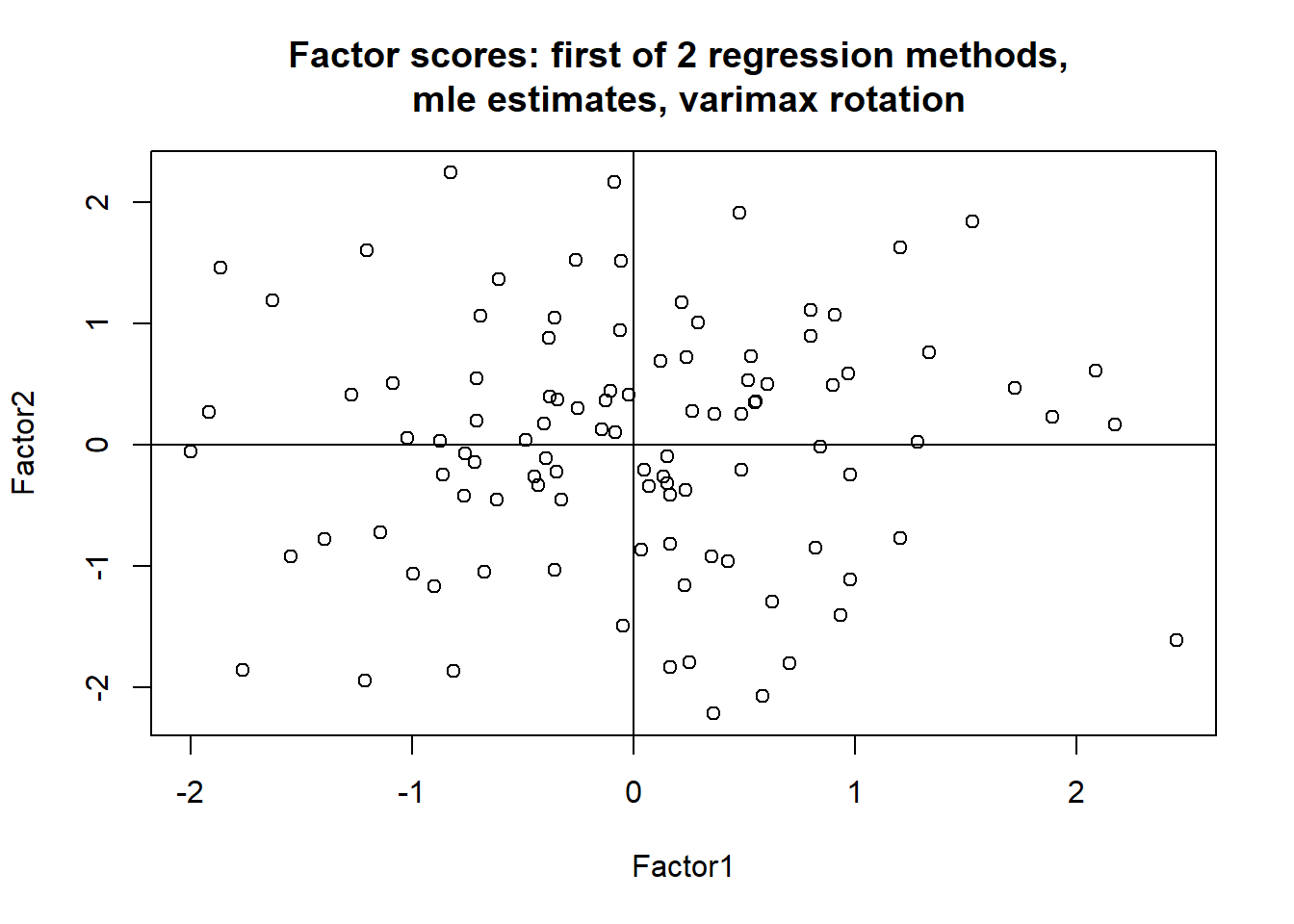
# Data reduction is accomplished by replacing the standardized data by these two simple factor scores.
plot(fit.ml.reg.r$scores, main = "Factor scores: first of 2 regression methods, \n mle estimates, varimax rotation")
abline(h=0)
abline(v=0)

2.7 Reference

[1] Johnson, R. A., and Wichern, D. W. (2007). Applied multivariate statistical analysis (6th ed.). Upper Saddle River, N.J.: Pearson Prentice Hall.

[2] Zelterman, D. (2015). Applied Multivariate Statistics with R (1st ed.).

[3] Statistics 575: Multivariate Analysis, Douglas Wiens (http://www.mathstat.ualberta.ca/~wiens/stat575/stat575.html)

1 Chapter 8: Principle Component Analysis

3 Chapter 10: Discrimination and Classification